
Balancing Transmission Line Ringing and Impedance Control in PCB Design
All traces will behave like transmission lines if long enough, and they can exhibit noticeable ringing when the rise time is very short (less than 1 ns). This will occur even if there is a perfect impedance match between the driver, trace, and receiver in a short line. In an electrically long line, there can still be some transient ringing from parasitics. Impedance matching requires precise trace design such that the trace impedance takes a specific value (usually 50 Ohms). However, the trace dimensions will determine the parasitic capacitance and inductance of the trace, which then determine the transmission line characteristic impedance, any ringing amplitude, and damping rate in your signals.
With single-ended impedance controlled traces, you need to carefully adjust the trace thickness, width, and distance from the reference plane in order to keep the impedance at a constant value while maximizing damping rate for any transient or reflective ringing. Ideally, you should get to critical damping as this will eliminate any transient oscillation in your board. Standard simulation tools for PCB design can help if you build the right model for your interconnects, although this requires extracting the parasitic capacitance and inductance per unit length in the interconnect.
Microstrip and symmetric stripline trace dimensions.
The same idea applies to differential impedance control and crosstalk in PCB design, but you need also need to account for the spacing between traces as this defines the differential impedance. In other words, you need to adjust the characteristic impedance of each line in the pair, as well as the coupling between pairs in order to adjust the ringing/damping and crosstalk susceptibility while maintaining a constant differential impedance. This is because differential signalling standards typically specify a specific differential impedance value rather than a characteristic impedance for routing.
This process can be difficult with differential transmission lines unless you know the coupling coefficient for the two lines in the pair. However, for single-ended microstrip or stripline transmission lines, you can use Wadell’s equations for the characteristic impedance alongside the approximate propagation delay, impedance in terms of parasitics, and propagation constant from the Telegrapher’s equations to size trace dimensions to maintain impedance while minimizing noise sources.
Example with Microstrip Traces
Let’s take a look at an example with single-ended microstrips and striplines. I’ll run through an example with microstrips, but you can take the same approach with single-ended striplines. To start, we need an accurate equation for the impedance of a single-ended microstrip trace. Wadell’s equations are widely regarded as the most accurate equations for describing the impedance of microstrip traces:

Eq. (1): Wadell’s equations for the impedance of microstrip traces.
Next, we need the signal velocity, which simply involves a conversion from the speed of light in vacuum to the speed of light in our particular substrate. Note that the dielectric constant seen by the signal is an effective dielectric constant due to the geometry of the microstrip, which is exposed to air at the top side.

Eq. (2): Signal velocity for microstrip and stripline traces in ps/inch.
Finally, we need two equations from the standard circuit model for transmission lines. Here, we are using the parasitic capacitance and inductance per unit length to define the trace impedance and signal velocity:
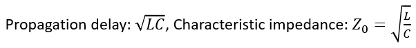
Eq. (3): Propagation velocity and characteristic impedance from the lumped transmission line circuit model.
As the damping in the line (according to RLC circuit theory) is inversely proportional to the parasitic inductance per unit length, your goal in reducing ringing as part of impedance control in PCB design is to maximize damping while minimizing the inductance per unit length in Eq. (3). This is done under the constraint that the characteristic impedance is held constant. Note that there are many other factors determining damping of any transients, as well as susceptibility to crosstalk and coupling strength to other lines.
This is a rather complex nonlinear optimization problem with three variables (the trace dimensions) and two constraints. One of these constraints is that the characteristic impedance be held constant, while the other depends on the ratio of the width of the trace to its height above the substrate (see Eq. (1)). This type of problem may be amenable to gradient descent methods, although my preferred method for this type of problem is to use an evolutionary algorithm. This type of algorithm is slower than gradient descent methods (e.g., generalized reduced gradient), but it is adaptable to strongly nonlinear problems. It can also be customized as a self-adaptive optimization algorithm, where the algorithm chooses among different population generation strategies as the algorithm runs.